Ph.D. Research

Drift-Diffusion Modeling of Solar Cells

Part of my Ph.D. research was on drift-diffusion modeling of solar cells. In particular, I focused on perovskite and organic solar cells but the modeling techniques are applicable to all semiconductor devices.

The basic components of a solar cell are two electrodes (at least one of which allows transmission of light) and an absorber/active layer which is made of a semiconductor. The working principle is based on the photovoltaic effect where photons of energy greater than the electronic bandgap of the absorber layer excite electrons from the valence band (VB) to the conduction band (CB), leaving behind holes (absense of an electron, which are treated as quasi-particles). Due to an energy level difference between the cathode and anode work functions, a solar cell has a built-in electric potential. Due to this potential and diffusion, the photogenerated free electrons and holes separate and move on average in opposite directions to the positive and negative contacts, thus generating a current. This current can be described as having contributions from drift due to the potential and diffusion due to the concentration gradient. The mechanism of separation of the electrons and holes is dependent on the materials and architecture of the cell.

Drift-diffusion modeling is the most popular approach for solar cell modeling due to its low computational cost (compared to other approaches) and good ability to explain and predict the experimentally measured performance of devices. The most simple drift diffusion modeling is done in 1 dimension along the dimension perpendicular to the electrodes and is often sufficient to represent a solar cell. In this approach, the 1D drift-diffusion Poisson equations are solved using finite differences and a special discretization scheme (Scharfetter-Gummel) to improve stability. The main result is usually in the form of a current-voltage curve, which is found by solving the equations at each applied voltage to find the current produced by the device. Thus, the current-voltage curve indicates the performance of the device: higher area under the curve means higher device efficiency. We can study the effects of various physical parameters on the performance using this model. An example of such a study is shown below.

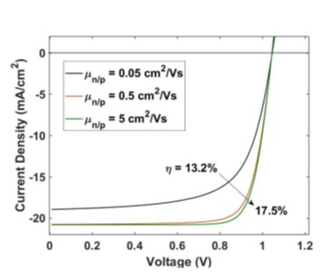
Figure: Example of the effect of carrier mobility on JV curve in a perovskite solar cell.

Equations Overview

In the device, the electric potential is due to the free electrons (n) and free holes (p) and is described by the 1D Poisson equation

$\frac{\partial ^2}{\partial x^2}\psi(x) = \frac{q}{\epsilon(x)}[n(x)-p(x)]$

where q is the elementary charge (always positive) and is the dielectric constant. The above equation is assuming that is constant within each layer of the device. The current density is separated for electrons and holes (Jn and Jp respectively) and related to the net free carrier generation rate U(x) by the continuity equations.

$\frac{\partial J_n}{\partial x}(x) = -qU(x)$

$\frac{\partial J_p}{\partial x}(x) = qU(x)$

The equations to find U generally involve using a transfer-matrix optical model to find the photogeneration rate and also considering charge recombination and dissociation rates. The specific equations will vary depending on the solar cell device which is being modeled. Recombination loss mechanisms can be electrons and holes recombining (bimolecular recombination) or electrons/holes recombining with defects(traps) in the material (Schockley-Read-Hall recombination). The current densities are also related to the electric potential and charge carrier densities through the drift-diffusion equations where Dn and Dp are the diffusion coefficients and are the charge carrier mobilities.

$J_n = -qn\mu_n\frac{\partial}{\partial x}\psi + q\mu_n V_t\frac{\partial}{\partial x}n$

$J_p = qp\mu_p\frac{\partial}{\partial x}\psi - q\mu_p V_t \frac{\partial}{\partial x}p$

Usually the where $V_t = k_B T/q$ is called the thermal voltage. The drift-diffusion and current continuity equations are usually combined.

The equations can be discretized using finite differences as follows. The Poisson equation is discretized using the central difference approximation for the 2nd derivative:

$\epsilon_i \frac{\psi_{i-1}-2\psi_i + \psi_{i+1}}{\delta x^2} = q(n_i - p_i)$

For the drift-diffusion equations, a special discretization approach called Scharfetter-Gummel is needed for the drift-diffusion equation in order to insure numerical stability.

$J_{n,i+1/2} = \frac{qV_tN\mu_{n,i+1}}{\delta x}(B(\delta \psi'_{i+1})n'_{i+1} - B(-\delta \psi'_{i+1})n'_{i})$

$J_{p,i+1/2} = -\frac{qV_tN\mu_{p,i+1}}{\delta x}(B(-\delta \psi'_{i+1})p'_{i+1} - B(\delta \psi'_{i+1})p'_{i})$

In a 1D model, the finite difference equations can be written as tridiagonal matrices which can be solved using simple techniques (i.e. Thomas algorithm). The Poisson and drift-diffusion matrix equations are solved in an iterative process in either a decoupled (Gummel method) or coupled (Newton-Raphson method) way until convergence is reached.

For some soler cells, such as bulk heterojunctions where there is a complex morphology of the device layers, a 2D drift-diffusion model may be desired to explore the effects of this morphology. The same equations can still be discretized in an analogous approach, but the resulting matrix equations are no longer tridiagonal which requires use more sophisticated solvers (i.e. bicongugate stabilized gradient BiCGSTAB method)

The model can also be extended to 3D which could be used to study situations where there is no 2D symmetry, such as simulating a conductive atomic force microscopy experiment which allows to measure local currents of solar cell materials. In this case we need to include the measuring probe which breaks the symmetry, requiring us to use a 3D model. A 3D model is quite computationally expensive due to the matrix equations which need to be solved become large (i.e. a small 20nm^3 region would be described by 8000x8000 matrices when using the typical 1nm mesh size). Such models need to be written in an efficient programming language such as C++ and the code must be optimized (one way is to use fast sparse matrix solvers such as BiCGSTAB). Parallelization should also be attempted.

This 3D model can be also used for modeling other electronic transport problems such as the current spreading from a conductive atomic force microscope tip.